Juan's RLAC Notes

---

A Distant Reading of War Letters

written with Aryamaan Dholakia

In this piece, we look at a collection of old books about war, and try to get to know more about the development of the war through a distant reading of what people who lived through it wrote. To achieve this, we sourced five collections of war letters from World War I written by English-speaking soldiers from the Internet Archive [link] and performed Optical Character Recognition on them using Tesseract [link]. With the resulting plain text, we first used sentiment analysis to gauge the overall change of the mood over the length of the books, and then used a comparative approach to look at the differences between the “more negative” and the “more positive” parts of the collections.

The books we sourced included an OCR layer added to them when they were digitalised (added with ABBYY FineReader). Looking at these results in contrast to the ones we generated with Tesseract, we found some differences that, if not accounted for, would make or break a distant reading of the texts.

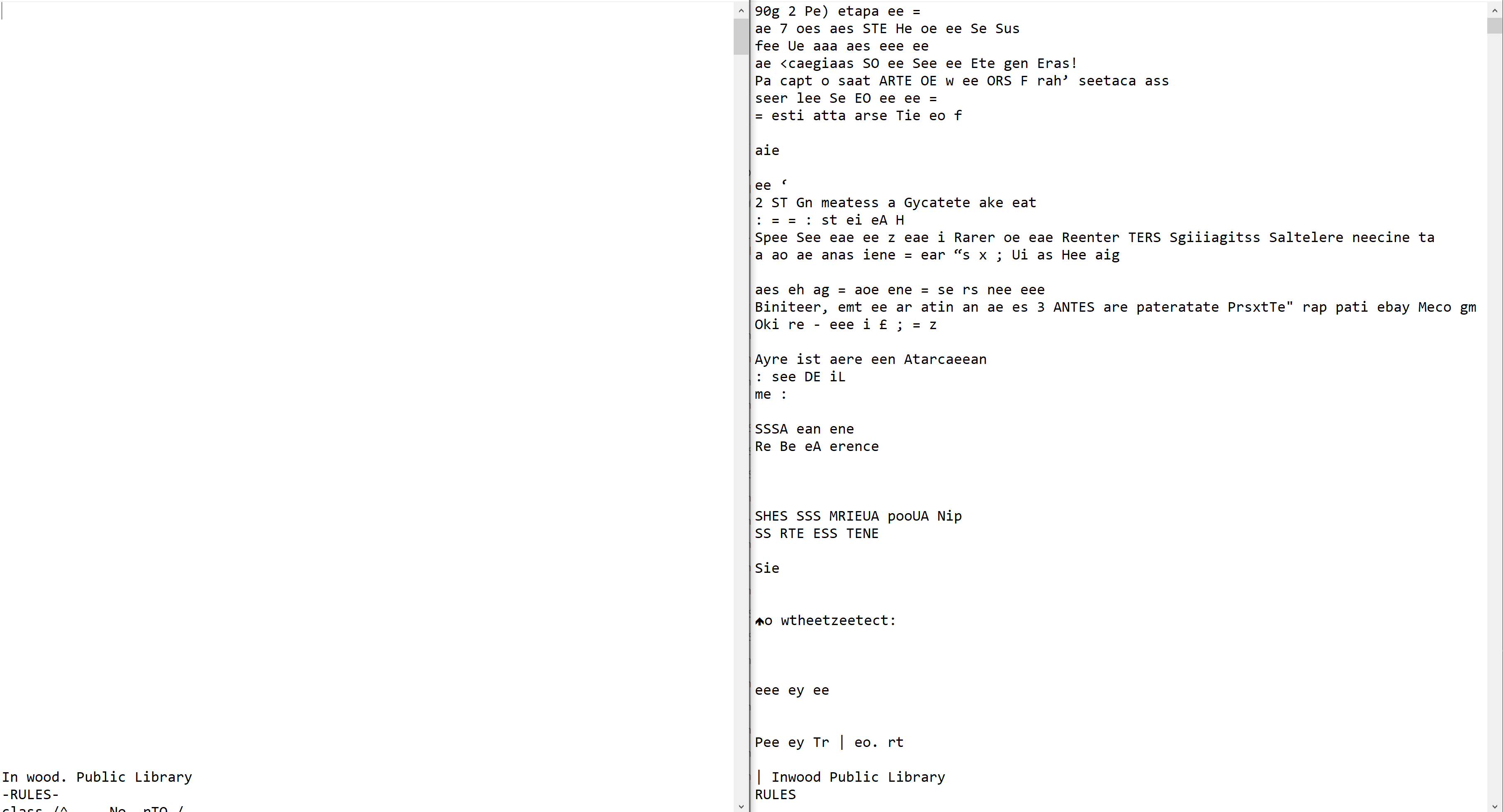
OCR results for the cover of "Carry On". To the left, the OCR packaged with the document. To the right, the Tesseract result.

Firstly, the OCR layer packaged with the texts encoded an entire page or block of text as a line in the file. This makes it difficult to divide the files into chunks of similar sizes for sentiment analysis as, for example, both the text “Page 96” and the entirety of Page 96 would be encoded equally as one line each in the output file. As R reads and labels text per line, this text would be divided in sectors with highly uneven sizes. Meanwhile, Tesseract’s OCR outputs text in a layout similar to that of the printed page, assigning one line in the file to every line in the output file and making it easier to manipulate it.

OCR results for the introduction of "Carry On". To the left, the OCR packaged with the document. To the right, the Tesseract result.

However, we noticed that Tesseract, as a general-purpose tool, didn’t perform as well as the original OCR (which could have been adjusted to recognise the text area of the particular books we analysed) at appropriately telling text and non-text (such as decorations, illustrations, and figures) apart. This makes the Tesseract-generated file have a lot more noise, however, if we use a bag-of-words approach, the noise won’t be picked up as a frequent word nor correspond to anything in a sentiment analysis lexicon, making the Tesseract OCR more annoying to read as a text file but easier to read for the computer.

We then decided to go ahead with the Tesseract-generated OCR for our analysis. For the first part of our exploration, we used R and the ‘bing’ [link] lexicon to perform a sentiment analysis of the books. To achieve this, we divided the books into chunks of 50 lines, and for each of these chunks we assigned a “negative” or “positive” value to each word that appears in the lexicon. Afterwards, we computed the total “sentiment value” per chunk as the total number of positive minus negative words. We plotted these values and calculated lines of best fit to identify trends in the development of the books.

Sentiment analysis results for the five books. Mostly positive books marked in green, mostly negative books marked red.

Our first observation from very lightly skimming the books [link] is that the letters are organised chronologically. Therefore, we could hypothesize that these graphs could, in a way, express the state of the war from the soldier’s perspective at different points in time. We first expected the books to have overwhelmingly negative scores, given that our lexicon would assign negative values to words related to war, violence, and sickness even if used in a positive context. However, we came to the surprising observation that two of the books were positive in the majority of their sectors, leading us to hypothesise that their authors might have focused their letters on topics of longing and home rather than describing the scenes of war.

Sentiment analysis results for the five books. Negative "dips" marked in red.

However, we also noted that most of the graphs have “dips” into negative values, this dip being around one quarter of the book in three of them. Have three of our authors, then, been a part of an especially intense period of the war that happened around its first quarter? We also see that another of the books presents a similar dip later: does this mean that this collection of letters ends prematurely and its dip corresponds chronologically to the other three? Or, on the contrary, was the author of this book on a different part of the war to the others, and therefore experienced a different period of increased violence?

Here is where a closer reading into the texts is essential to clear this kind of doubts. The text with the anomalous “dip” is “War Letters from a Public-School Boy” [link], which, on closer reading of its table of contents [link], we find out is divided in two sections, each taking roughly half of the book: one of pre-war letters and other of letters during the war. If we ignore the first part of this book, then, we can notice the “dip” occurs in a similar place to the other books.

If we assume that the collections have letters from the start to the finish of the war in a roughly evenly distributed frequency, we could hypothesise that around the second quarter of the war (in terms of time, around the Spring of 1916) there was a period of intensified violence that most of our authors witnessed and wrote about. However, a closer reading of the texts and the dates of the letters in the sectors that form the “dip” and a mapping into actual battle events is necessary to confirm this hypothesis.

Because this is distant reading and we don’t do that here [link to sth funny], we decided to use AntConc to contrast the “worst” and the “less bad” parts of the books as returned by our sentiment analysis. Given that the first half of the books usually consist of more ‘negative’ emotions compared to the latter half of the books, we decided to build two corpora: one with the first halves of the books and another with the second halves, and contrasted them.

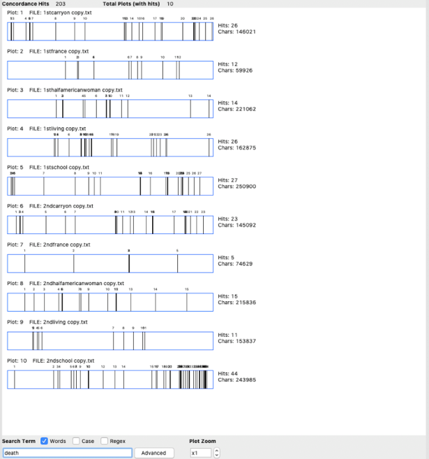
Our analysis started with a fascinating finding: that though the second half of the books was more “positive” in the sentiment analysis, it contained a higher frequency of words that are usually associated with negativity. Words like “war,” “death,” “kill” and “dead” all had a higher frequency in the second half than the first.

Concordance plot for “death” highlighting greater frequency in the second halves (bottom 5 rows).

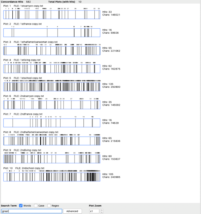
Concordance plot for “great” highlighting an almost equal frequency in both halves.

The question then arose: why, then, did our sentiment analysis output that the second half of the books were more positive than the first? One possible hypothesis could be the presence of several more positive words in the second half as compared to the first, but when put to the test with words such as “great,” “love,” “good,” “happy” and “sad” the frequency was relatively the same across the first and second halves of the books. We then proceeded to compare the most frequent words generally associated with positivity or negativity in each half, obtaining the following results:

As observed above, the most frequent words are exactly the same. The difference between the two columns is the position of “love”. In the first half, “love” stands at 5th while it’s at 3rd in the second half. This could lead to a hypothesis highlighting the importance of collocation in sentiment analysis: positive words in the lexicon used will not have a great effect on the output per sector if they are grouped with negative words, and given that this grouping is almost entirely dependent on the granularity of the sectors, different partitions of the books could be able to return different results per sector. This makes our sentiment analysis also unable to determine the effects of proximity between negative and positive words, as their contrast could be used to intensify the effect of either of them.

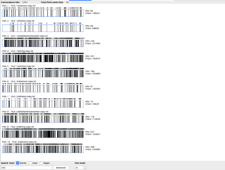
For example, we could see the importance of the particle “not”. Consider the sentence “I am not very good”. Any primitive sentiment analysis approach would just flag this sentence positive because of the word ‘good’ that apparently would appear in the positive dictionary. But reading this sentence we know this is not a positive sentence. “Not” is used more frequently in the second half than the first, which could be a reason for the second halves to be considered more positive by our sentiment analysis when they might actually be as negative as the first halves. However, when we used collocates to confirm this idea, there were only a handful of instances that the word “not” appeared before a positive word, invalidating this idea.

Concordance Plot of “not” highlighting higher frequency in the second half (bottom 5 rows).

Then why does our AntConc analysis not agree with the graphs we observe using sentiment analysis? Pinpointing the words identified by R in the text, based on the lexicon incorporated, could be an interesting start point for this investigation. Additionally, we can also consider that as for we analysed each text individually in our sentiment analysis, while in AntConc we created a corpus of all the first halves of the books and all the second halves, the relative effect of the positive and negative words might have been impacted.

Also, given the books are of different sizes, a longer book that goes against the general trend could have had a heavier effect on the analysis. Moreover, this may have resulted in our corpus being overlapped with different time periods: for instance, if the books were written in chronological order, the halfway mark for some books may coincide with the year 1916 while others may coincide with 1917. An effective way to solve this issue would have been to create a halfway point ourselves, say the end of 1916 and segregate the corpus with the first half of the texts being written before 1916 and the second half after 1916.

Therefore, it is quite clear that there are several factors that dictate sentiment analysis that are not simply limited to a positive or negative emotional index as rated by our use of a lexicon, but may also include frequency of the words and their relative impact on each other. This analysis should be extended to the context in which the words are used in, to improve accuracy, which could be done by analysing the collocates of the words along with their definitions. The one thing that can be concluded from this analysis, though, is that the OCR itself proved to be extremely accurate, providing differences only in the spacing of the text, and with proper management didn’t impact our analysis heavily.

See the R notebook for this assignment.
Download the AntConc screenshots.

ready for grading - november 23th, 2021